|
  x0 = (blk[8*0]<<8) + 8192;

  /* first stage */
  x8 = W7*(x4+x5) + 4;
  x4 = (x8+(W1-W7)*x4)>>3;
  x5 = (x8-(W1+W7)*x5)>>3;
  x8 = W3*(x6+x7) + 4;
  x6 = (x8-(W3-W5)*x6)>>3;
  x7 = (x8-(W3+W5)*x7)>>3;

  /* second stage */
  x8 = x0 + x1;
  x0 -= x1;
  x1 = W6*(x3+x2) + 4;
  x2 = (x1-(W2+W6)*x2)>>3;
  x3 = (x1+(W2-W6)*x3)>>3;
  x1 = x4 + x6;
  x4 -= x6;
  x6 = x5 + x7;
  x5 -= x7;

  /* third stage */
  x7 = x8 + x3;
  x8 -= x3;
  x3 = x0 + x2;
  x0 -= x2;
  x2 = (181*(x4+x5)+128)>>8;
  x4 = (181*(x4-x5)+128)>>8;

  /* fourth stage */
  blk[8*0] = iclp[(x7+x1)>>14];
  blk[8*1] = iclp[(x3+x2)>>14];
  blk[8*2] = iclp[(x0+x4)>>14];
  blk[8*3] = iclp[(x8+x6)>>14];
  blk[8*4] = iclp[(x8-x6)>>14];
  blk[8*5] = iclp[(x0-x4)>>14];
  blk[8*6] = iclp[(x3-x2)>>14];
  blk[8*7] = iclp[(x7-x1)>>14];
|
|
|
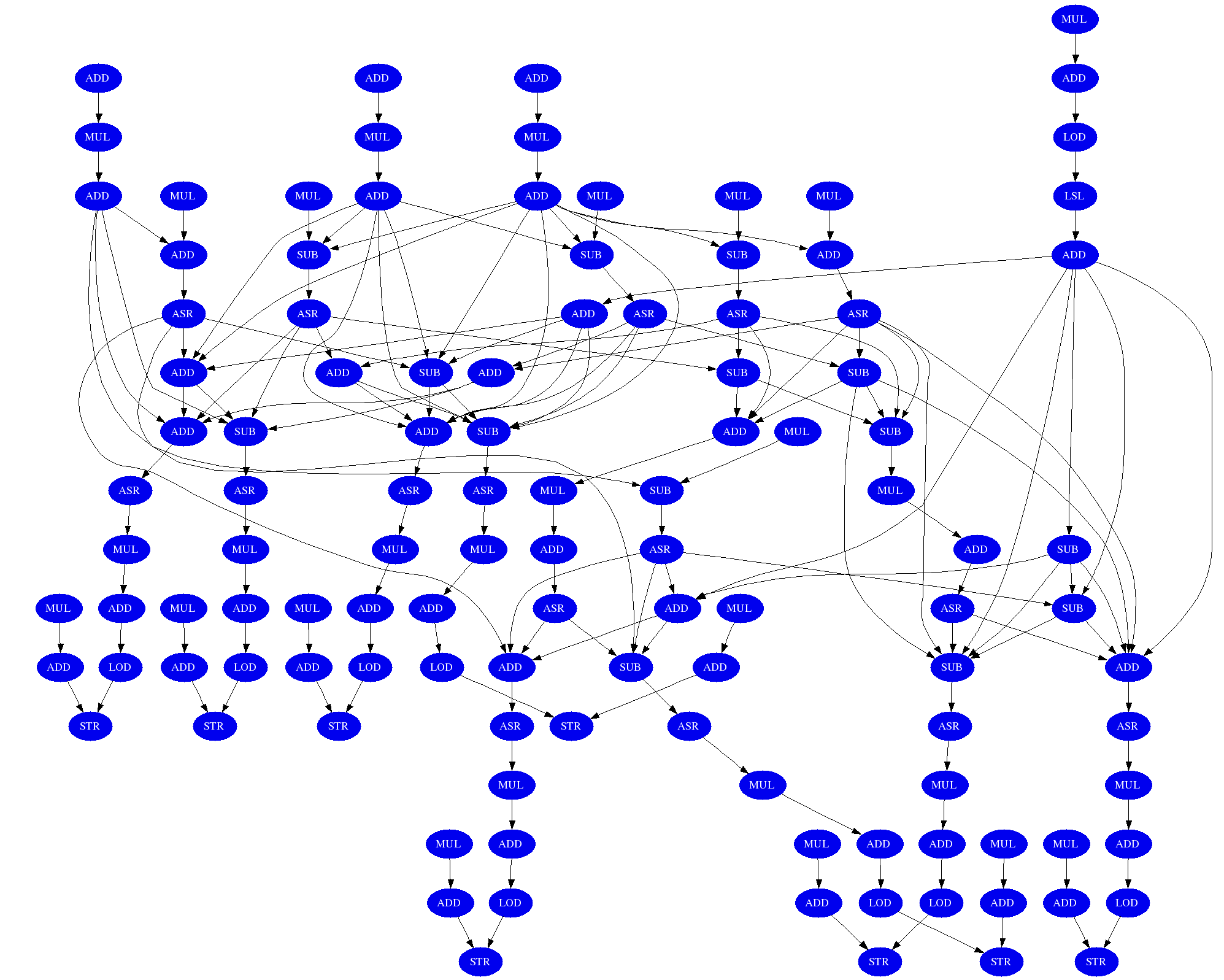
The inverse discrete cosine transform function was selected to contrast the implementation
in the JPEG application. The idct DFG has a large number of nodes, which again helps to
stress test the scheduling algorithm.